AVISO
About
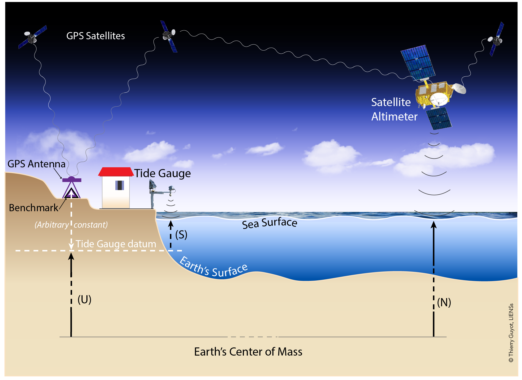
In briefest terms, the approach consists in differencing the sea level time series from a tide gauge with an equivalent time series from satellite altimetry. To the extent that both instruments measure identical ocean signals, their difference is a proxy for the vertical position of the tide gauge. Assuming that the instrumental drifts are negligible, the time series of the sea level differences will then be dominated by vertical land motion at the tide gauge. This is illustrated in the figure on the right (click on the image to enlarge).
It is essential that the processing of both data types be as consistent as possible too. For instance, since an atmospheric correction is typically applied to satellite altimetry data, we applied the identical correction to the tide-gauge data. This correction is referred to as SLP (Sea Level Pressure) correction in the header of the t-files, but it comprises the static and dynamic effects of the atmosphere. The corrections were provided by AVISO under the name Dynamic Atmospheric Correction (DAC). However, the details of the atmospheric corrections and their accuracies are not relevant here, since common errors will cancel in the differentiation. It is the consistency of models and corrections applied to both datasets that must be ensured.
– Tide gauge data:
All tide gauge data used in our calculations are from the Revised Local Reference (or ’RLR’) dataset of the PSMSL. We selected tide gauges with more than 15 years and a minimum of 70% of valid monthly mean sea levels over the satellite altimetry period, starting in 1993.0.
– Satellite altimetry data:
We used time series of satellite altimetry mean sea level anomalies (SLA), i.e., sea surface heights with respect to an arbitrary temporal mean (it can be different from one provider to the other), whose primary raison d’être is to avoid large numerical values (decametric ellipsoidal heights with regard to the expected centimeter level changes in mean sea levels). Note that we considered satellite altimetry data from several data suppliers.
Here, we are dealing with the data set identified as Global MSLA heights in delayed time ("all sat merged") from the Archiving, Validation, and Interpretation of Satellite Oceanographic data (AVISO; http://www.aviso.altimetry.fr/en/data.html). The temporal sampling was homogenized to time series of monthly data.
– Sea level differences:
Time series of sea level differences (SLD) between monthly tide gauge and satellite altimetry data were built using three variants of satellite SLA time series, namely the closest grid point, the most correlated grid point, and the average within a 1° radius from the tide gauge location. However, since the differences between these variants were negligible, we adopted the SLA averaged within a radius of 1° around the tide gauge location.
Once computed, the time series of sea level differences (SLD) were checked visually to discard those that displayed clear non linear behaviour, i.e., for which vertical land motion would not be adequately modelled by a linear trend. We then estimated the linear trend of the de-seasoned and de-trended SLD time series. All quoted uncertainties represent 1-sigma standard errors.
– Future updates:
We plan to update the calculations of the sea level differences on a yearly basis, because as the time series lengthen and the satellite providers improve their products (new models, corrections, algorithms...), some level of improved precision is expected. However, there can be real differences between sea levels measured by a tide gauge at the coast and that measured off-shore by a satellite altimeter, due to the ocean processes which occur between the two points. This could be interesting to investigate and monitor. By contrast, for most open ocean locations, there is usually a high degree of correlation between variability in the two types of sea level. In this case, the vertical land motion can be estimated, provided the instrumental drifts are negligible. If there are (drifts), it enables tide gauge data to be used as a check on the satellite altimeter information and its stability and, conversely, it enables gross errors in tide gauge datum to be identified.
Download
The web map enables the users to navigate from one site (station) to another, and click on a specific site in the map to see its attributes. By clicking further, an individual web page for the site can be accessed, where details on the data and meta-data are displayed for that site. The user can then get some additional statistics and download files with the associated time series (sea level differences...). Here, we provide a more comprehensive means to download the data from all the sites.
– Table of linear trends of sea level differences
The vertical_velocities_ALTG_AVISO.txt provides the vertical velocities and uncertainties for the 478 stations for which we computed the monthly sea level differences (satellite altimetry minus tide gauge data) and derived a linear trend (see About).
– Time series of monthly sea level differences
The useries_aviso.zip archive (.zip file) contains the 478 individual files of monthly sea level differences (satellite altimetry minus tide gauge data) time series. The format of the individual files is rather straightforward. The values are expressed in millimetres with respect to an arbitrary datum. The choice of the datum was arbitrary to avoid negative values (a constant of about 7000 mm was added to the differences).
Citation
G. Wöppelmannn & M. Marcos (2016) : Vertical land motion as a key to understanding sea level change and variability. Reviews of Geophysics, 54, pp. 64-92.


